Station 05 · diffusion
The Denoising Deck
Every image a diffusion model has ever made started as pure static. The deck below is a real Stable Diffusion 1.5 run — sampled on this site's own GPU, every intermediate state kept — so you can scrub the moment an image condenses out of noise, and catch the model guessing the ending long before it gets there.
instrument live — scrub the run · switch views · compare seeds
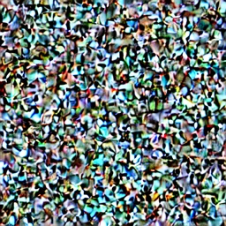
every state of this run
x_t — what the latent actually holds right now. same prompt, same model — only the starting noise differs between seeds.
prompt: “a lighthouse on a rocky cliff at dusk, dramatic golden clouds, crashing waves, oil painting” · 20 ddim steps · cfg 7.5
fig. 01 — one ddim run, 21 states, three ways to look at each
Noise is the curriculum
Diffusion training never shows the model how to paint — it shows it ruined paintings. Take an image, mix in gaussian noise at a randomly chosen severity t, and ask one question: “what noise was added?” The schedule ᾱ controls severity: near t=0 the image is barely touched, near t=1000 nothing of it survives. One network learns the whole range — denoising a nearly-clean image teaches texture, denoising near-static teaches composition.
The figure runs the real corruption formula on a toy scene. Notice the curve: destruction is scheduled, not linear — ᾱ falls slowly at first, then dives. And because the closed form jumps straight to any t, training never has to walk there step by step. That convenience is the whole reason the math works at scale.
xt = √ᾱ·x₀ + √(1−ᾱ)·ε — computed live, per pixel
same ε the whole way — drag t and watch structure drown gradually, not all at once
Sampling runs the film backwards
Generation is the inverse loop: start from pure noise, and twenty-odd times in a row, predict the noise and remove a scheduled slice of it. That’s the loop your ComfyUI KSamplerThe recipe deciding how big each denoising step is and how many to take (DDIM, Euler, and friends). runs, and it’s what the deck’s canvas view shows: the actual state, still snowy until surprisingly late.
The deck’s guess view is the revealing one. Because the model predicts the noise, you can algebraically peek at what it currently believes the finished image is — by state 5 of 20 it has already committed to a lighthouse, a cliff, and a dusk sky, and the remaining steps only sharpen the verdict. Composition is decided early at high noise; detail is negotiated late at low noise. That’s also why so many ComfyUI tricks — refiners, hi-res passes, prompt scheduling — split the run into an early “layout” phase and a late “rendering” phase.
The prompt's volume knob
Station 04 showed where the prompt enters: cross-attention, the denoiser reading your words through CLIP. Classifier-free guidanceClassifier-free guidance: the knob deciding how hard each denoising step is pulled toward your prompt. decides how loudly. Each step the model predicts twice — once with your prompt, once with an empty one — and CFG extrapolates past the unconditioned guess in the direction your prompt pulls: output = uncond + cfg·(cond − uncond).
The strip is the same starting noise at four volumes. At 1 the prompt is a whisper and the model paints whatever the noise suggested. At 12 every step is yanked so hard toward “lighthouse, dramatic, golden” that contrast clips and sameness sets in. The 7–8 default is a truce, not a law — knowing what the knob actually does is what lets you break it on purpose.
the everyday default
Latent space is a place
None of this happens on pixels. A VAEThe encoder/decoder pair that squeezes images into the compact working format and inflates results back to pixels. compresses each 512×512 image into the 64×64×4 tensorJust a grid of numbers — possibly with more than two dimensions. you saw in the deck’s raw latent view — 48× smaller — and the U-NetThe network shape doing the denoising work in Stable Diffusion — it sees the image at several zoom levels at once. denoises there; only the final latentA compressed stand-in for an image: a much smaller grid of numbers the model works on instead of raw pixels. gets decoded back to pixels. That compression is why this runs on a desktop GPU at all, and it’s the “latent” in latent diffusion.
The walk shows the deeper property: interpolate between two seeds’The number that picks the starting static — same seed, same prompt, same settings → the exact same image. starting noise and sample each point fully, and every stop along the path is a coherent scene — the lighthouse relocates, the clouds renegotiate, nothing ever tears. Generative latent spaces aren’t lookup tables of memorized images; they’re smooth maps where neighborhoods mean something. Station 01’s nearest-neighbor lab had no such geometry — this is what eighty pages of gradient descent buys.

the starting noises are interpolated (slerp), then each point is sampled fully — no crossfade anywhere, every frame is its own run
LoRA: fine-tuning on a budget
Teaching a checkpoint a new style shouldn’t require rewriting all 860 million weights, and LoRAA small add-on file that nudges a big model's weights toward a new style — learned cheaply by betting the change is simple.’s bet is that it doesn’t: the change a fine-tune needs is low-rankHow many independent directions a grid of numbers really uses — low rank means a few patterns explain almost everything. — a coordinated nudge along a few directions, not 860M independent edits. So instead of learning ΔW directly, a LoRA learns two skinny matrices A and B whose product is the update, at a tiny fraction of the parameters.
The lab makes that bet visceral with a 16×16 “update”: slide the rank and watch the bolt survive at r=3 — 96 numbers doing the work of 256. Scale the same ratio to a U-Net’s attention layers and you get the 10–200 MB LoRA files in your ComfyUI folder standing in for multi-gigabyte checkpoints. Every slider you’ve dragged on this site — k, learning rate, heads, rank — has been the same lesson: capacity is a dial, and knowing where it lives is the skill.
full ΔW (16×16 = 256 numbers)
rank 3: A(16×3) · B(3×16) = 96
most of the bolt survives at rank 3 — structured changes are low-rank, which is the entire bet a lora makes about fine-tuning
all five instruments live
That’s the journey: a line through a cloud of points, bent by activations, composed into vision, bound by attention, and finally run in reverse until static becomes a lighthouse. The best next instrument is a real one — open ComfyUI and watch these ideas operate at full scale.